Plots for Regression Predictions

Visualizations for mlr3::PredictionRegr. The argument type controls what kind of plot is drawn. Possible choices are:

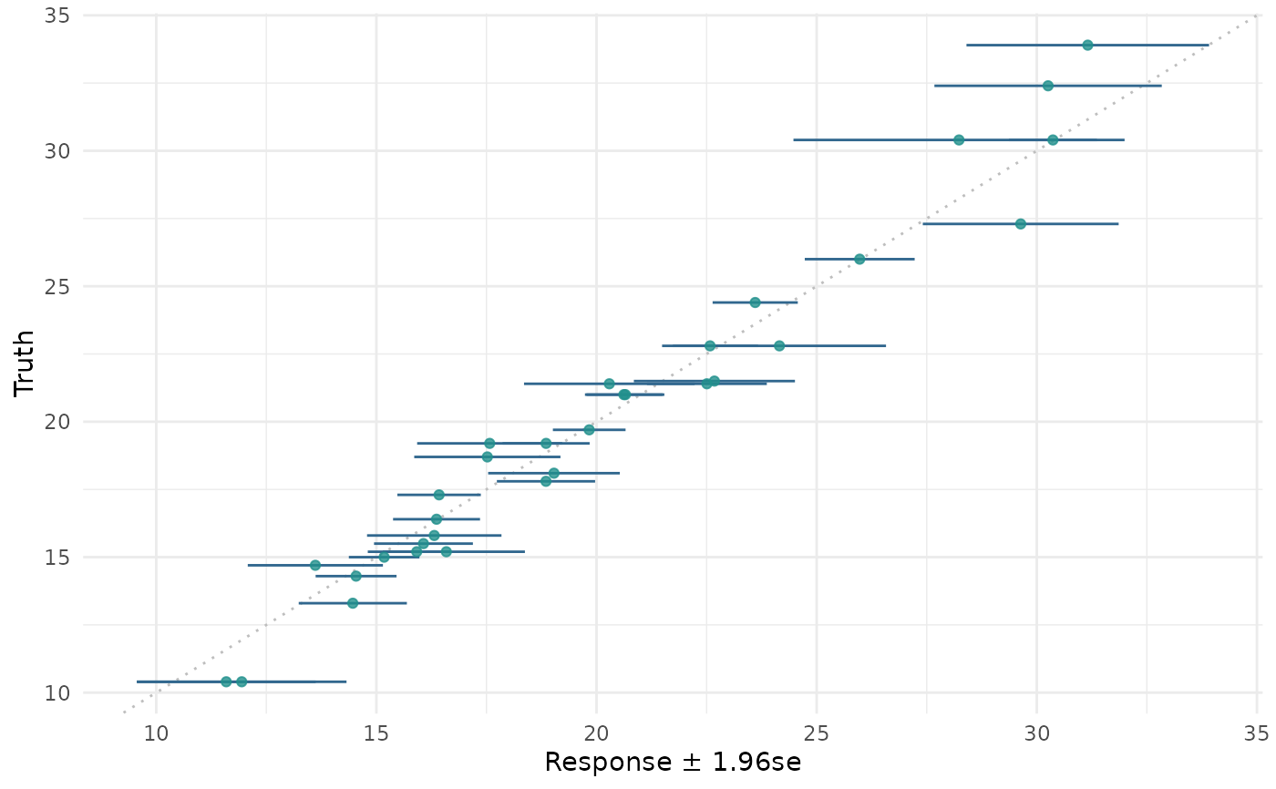
• "xy" (default): Scatterplot of "true" response vs. "predicted" response. By default a linear model is fitted via geom_smooth(method = "lm") to visualize the trend between x and y (by default colored blue). In addition geom_abline() with slope = 1 is added to the plot. Note that geom_smooth() and geom_abline() may overlap, depending on the given data.

• "histogram": Histogram of residuals: \(r = y - \hat{y}\).

• "residual": Plot of the residuals, with the response \(\hat{y}\) on the "x" and the residuals on the "y" axis. By default a linear model is fitted via geom_smooth(method = "lm") to visualize the trend between x and y (by default colored blue).

• "confidence: Scatterplot of "true" response vs. "predicted" response with confidence intervals. Error bars calculated as object$reponse +- quantile * object$se and so only possible with predict_type = "se". geom_abline() with slope = 1 is added to the plot.

Usage

# S3 method for PredictionRegr
autoplot(
  object,
  type = "xy",
  binwidth = NULL,
  theme = theme_minimal(),
  quantile = 1.96,
  ...
)

Arguments

object

(mlr3::PredictionRegr).

type

(character(1)):
Type of the plot. See description.

binwidth

(integer(1))
Width of the bins for the histogram.

theme

(ggplot2::theme())
The ggplot2::theme_minimal() is applied by default to all plots.

quantile

(numeric(1))
Quantile multiplier for standard errors for type="confidence". Default 1.96.

...

(ignored).

Value

ggplot2::ggplot().

Examples

if (requireNamespace("mlr3")) {
  library(mlr3)
  library(mlr3viz)

  task = tsk("boston_housing")
  learner = lrn("regr.rpart")
  object = learner$train(task)$predict(task)

  head(fortify(object))
  autoplot(object)
  autoplot(object, type = "histogram", binwidth = 1)
  autoplot(object, type = "residual")

 if (requireNamespace("mlr3learners")) {
  library(mlr3learners)
  learner = lrn("regr.ranger", predict_type = "se")
  object = learner$train(task)$predict(task)
  autoplot(object, type = "confidence")
 }
}