Plots for Optimization Instances

Visualizations for bbotk::OptimInstanceSingleCrit. The argument type controls what kind of plot is drawn. Possible choices are:

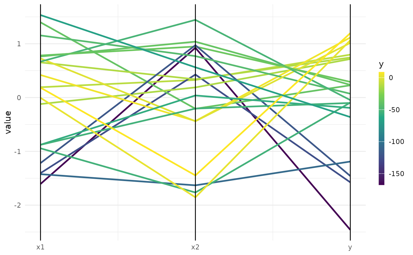
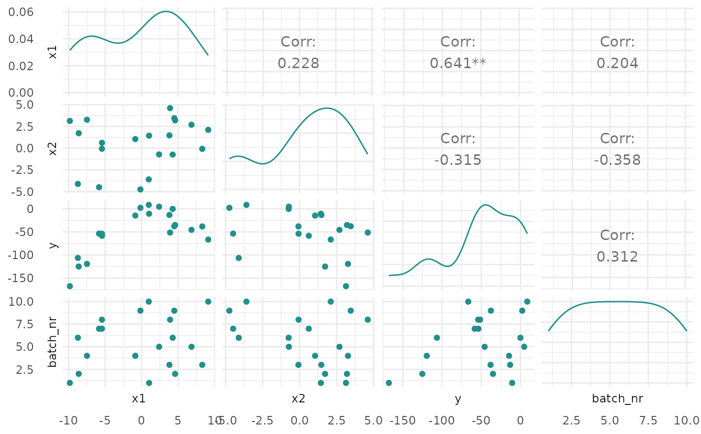
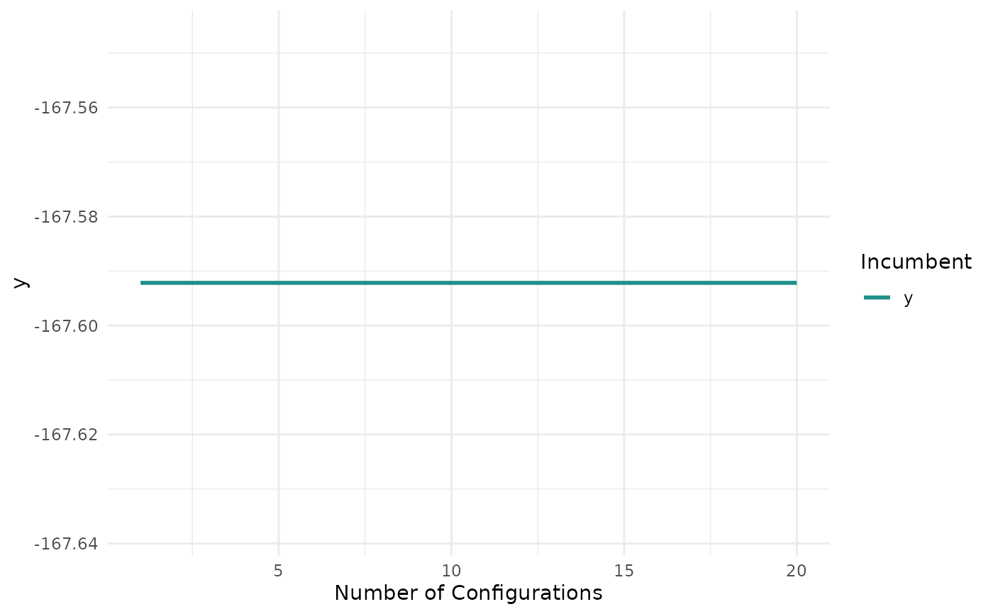
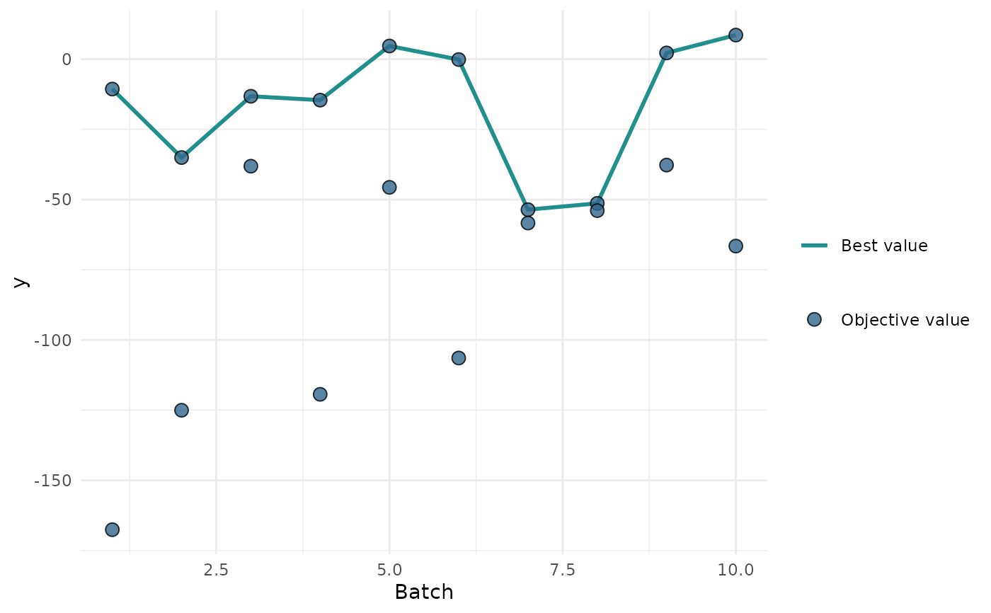
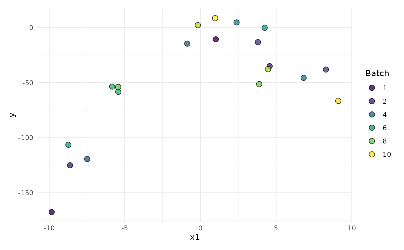
• "marginal" (default): Scatter plots of x versus y. The color of the points shows the batch number.

• "performance": Scatter plots of batch number versus y

• "parameter": Scatter plots of batch number versus input. The color of the points shows the y values.

• "parallel": Parallel coordinates plot. x values are rescaled by (x - mean(x)) / sd(x).

• "points": Scatter plot of two x dimensions versus. The color of the points shows the y values.

• "surface": Surface plot of two x dimensions versus y values. The y values are interpolated with the supplied mlr3::Learner.

• "pairs": Plots all x and y values against each other.

• "incumbent": Plots the incumbent versus the number of configurations.

Usage

# S3 method for OptimInstanceSingleCrit
autoplot(
  object,
  type = "marginal",
  cols_x = NULL,
  trafo = FALSE,
  learner = mlr3::lrn("regr.ranger"),
  grid_resolution = 100,
  batch = NULL,
  theme = theme_minimal(),
  ...
)

Arguments

object

(bbotk::OptimInstanceSingleCrit).

type

(character(1)):
Type of the plot. See description.

cols_x

(character())
Column names of x values. By default, all untransformed x values from the search space are plotted. Transformed hyperparameters are prefixed with x_domain_.

trafo

(logical(1))
If FALSE (default), the untransformed x values are plotted. If TRUE, the transformed x values are plotted.

learner

(mlr3::Learner)
Regression learner used to interpolate the data of the surface plot.

grid_resolution

(numeric())
Resolution of the surface plot.

batch

(integer())
The batch number(s) to limit the plot to. The default is all batches.

theme

(ggplot2::theme())
The ggplot2::theme_minimal() is applied by default to all plots.

...

(ignored).

Value

ggplot2::ggplot().

Examples

if (requireNamespace("mlr3") && requireNamespace("bbotk") && requireNamespace("patchwork")) {
  library(bbotk)
  library(paradox)

  fun = function(xs) {
    c(y = -(xs[[1]] - 2)^2 - (xs[[2]] + 3)^2 + 10)
  }
  domain = ps(
    x1 = p_dbl(-10, 10),
    x2 = p_dbl(-5, 5)
  )
  codomain = ps(
    y = p_dbl(tags = "maximize")
  )
  obfun = ObjectiveRFun$new(
    fun = fun,
    domain = domain,
    codomain = codomain
  )

  instance = OptimInstanceSingleCrit$new(objective = obfun, terminator = trm("evals", n_evals = 20))

  optimizer = opt("random_search", batch_size = 2)
  optimizer$optimize(instance)

  # plot y versus batch number
  print(autoplot(instance, type = "performance"))

  # plot x1 values versus performance
  print(autoplot(instance, type = "marginal", cols_x = "x1"))

  # plot parallel coordinates plot
  print(autoplot(instance, type = "parallel"))

  # plot pairs
  print(autoplot(instance, type = "pairs"))

  # plot incumbent
  print(autoplot(instance, type = "incumbent"))
}
#> Loading required namespace: patchwork
#> Loading required package: paradox


#> Registered S3 method overwritten by 'GGally':
#>   method from   
#>   +.gg   ggplot2